Time Series Prediction for Individual Household Power
Dateset: https://archive.ics.uci.edu/ml/datasets/individual+household+electric+power+consumption
The data was collected with a one-minute sampling rate over a period between Dec 2006
and Nov 2010 (47 months) were measured. Six independent variables (electrical quantities and sub-metering values) a numerical dependent variable Global active power with 2,075,259 observations are available. Our goal is to predict the Global active power into the future.
Here, missing values are dropped for simplicity. Furthermore, we find that not all observations are ordered by the date time. Therefore we analyze the data with explicit time stamp as an index. In the preprocessing step, we perform a bucket-average of the raw data to reduce the noise from the one-minute sampling rate. For simplicity, we only focus on the last 18000 rows of raw dataset (the most recent data in Nov 2010).
A list of python files:
- Gpower_Arima_Main.py : The executable python program of a univariate ARIMA model.
- myArima.py : implements a class with some callable methods used for the ARIMA model.
- Gpower_Xgb_Main.py : The executable python program of a tree based model (xgboost).
- myXgb.py : implements some functions used for the xgboost model.
- lstm_Main.py : The executable python program of a LSTM model.
- lstm.py : implements a class of a time series model using an LSTMCell. The credit should go to https://github.com/hzy46/TensorFlow-Time-Series-Examples/blob/master/train_lstm.py
- util.py : implements various functions for data preprocessing.
- Exploratory_analysis.py : exploratory analysis and plots of data.
+ Environment : Python 3.6, TensorFlow1.4.
Here, I used 3 different approaches to model the pattern of power consumption.
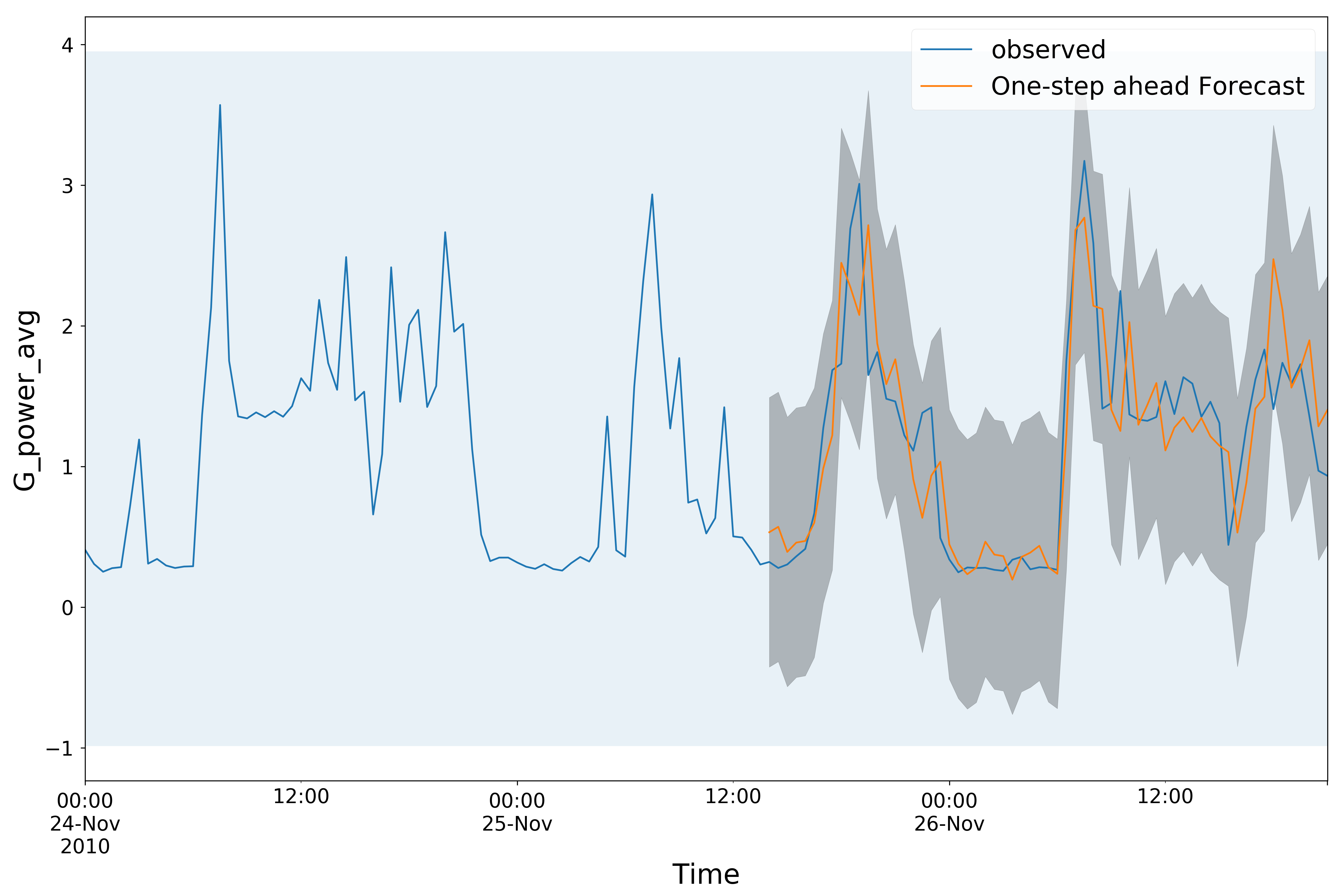
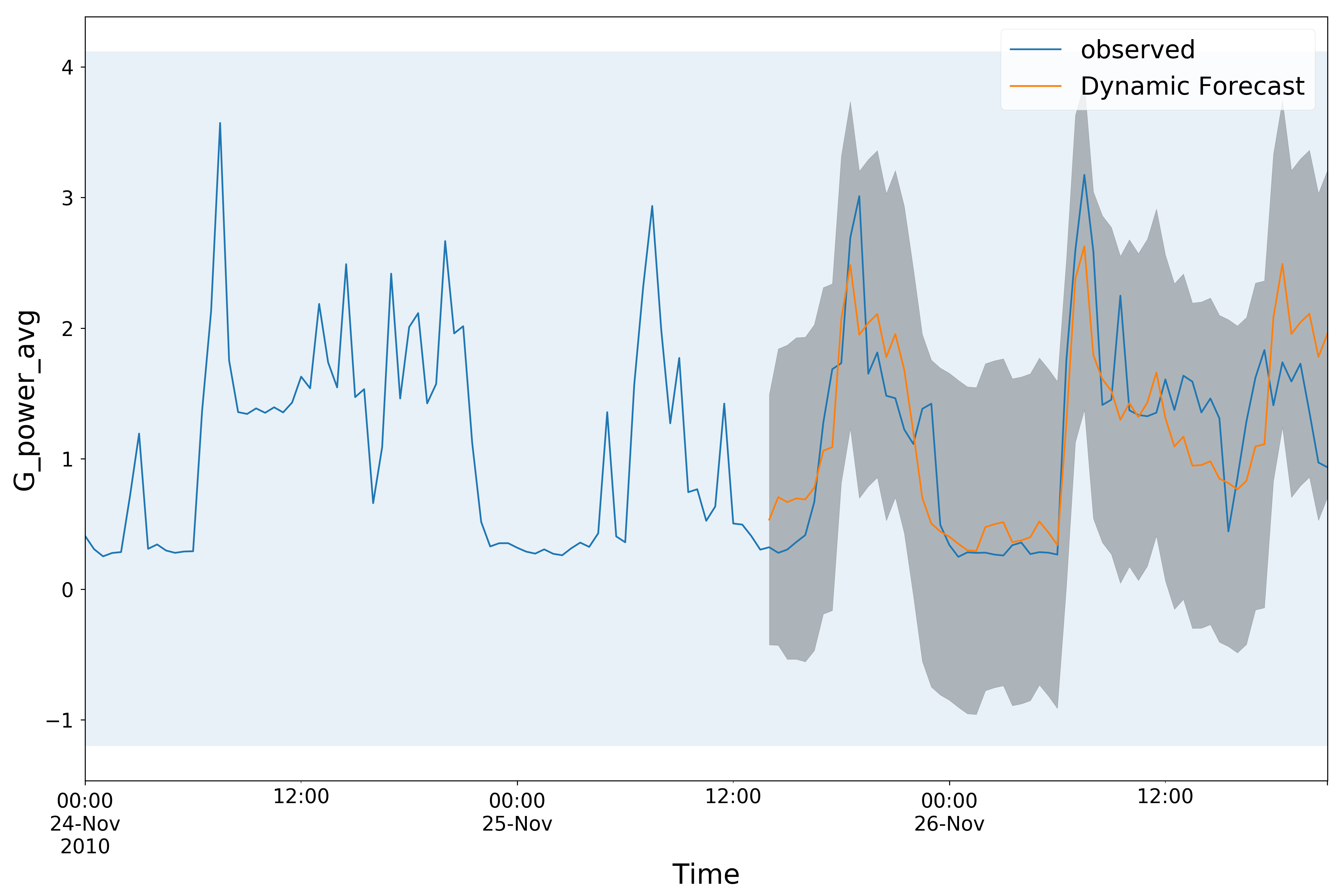
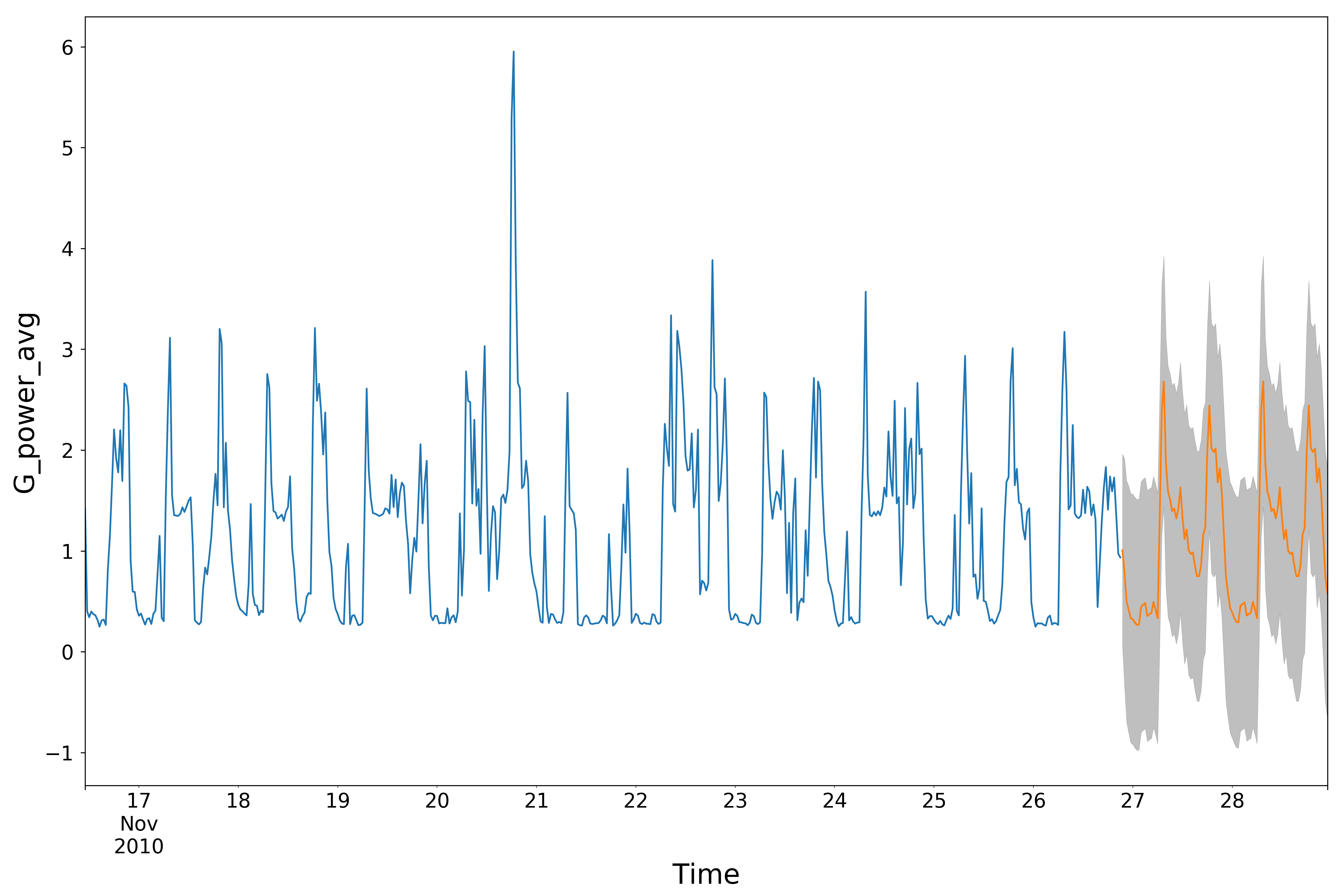
- Univariate time series ARIMA.(30-min average was applied on the data to reduce noise.)
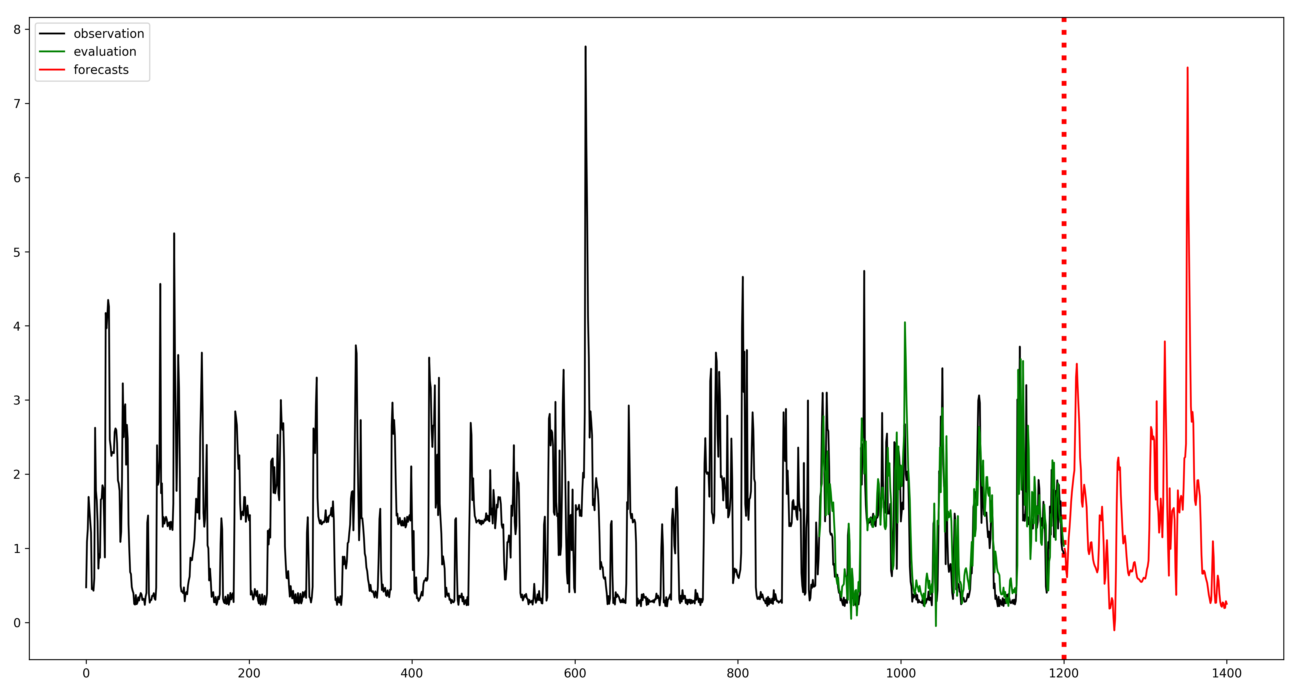
- Regression tree-based xgboost.(5-min average was performed.)
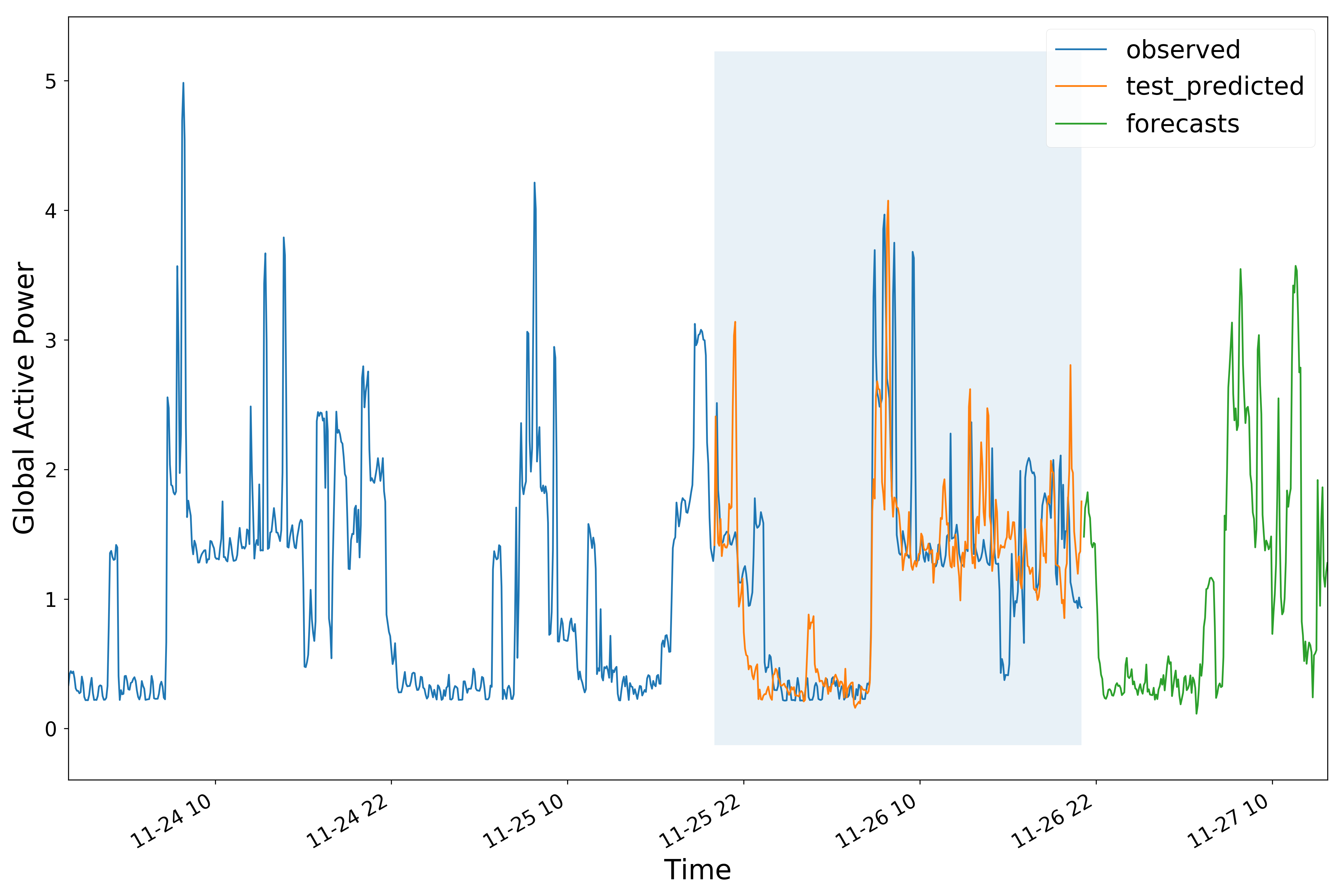
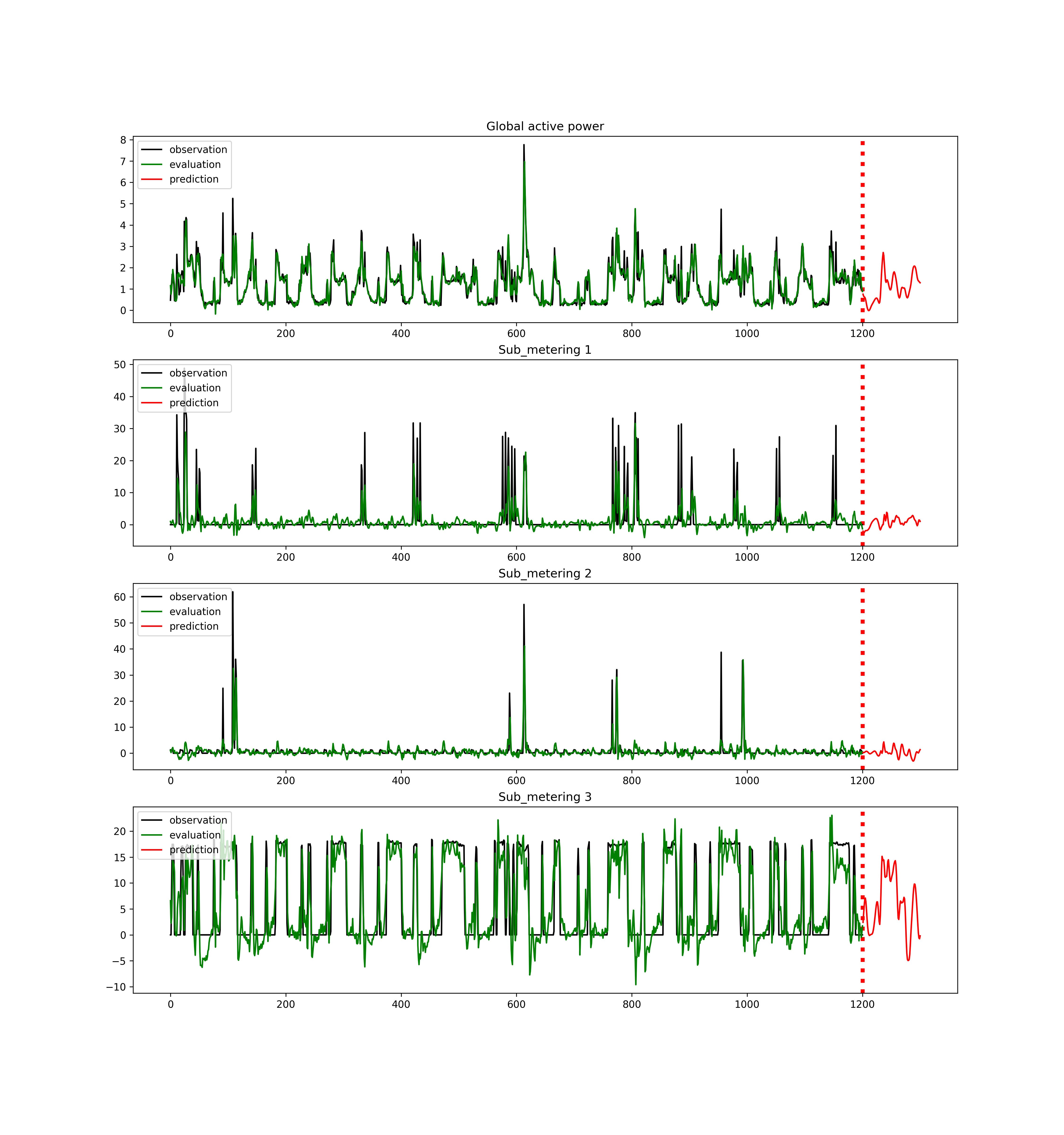
- Recurrent neural network univariate LSTM (long short-term memoery) model. (15-min average was performed to reduce the noise.)
Possible approaches to do in the future work:
(i) Dynamic Regression Time Series Model
Given the strong correlations between Sub metering 1, Sub metering 2 and Sub metering 3 and our target variable,
these variables could be included into the dynamic regression model or regression time series model.
(ii) Dynamic Xgboost Model
Include the timestep-shifted Global active power columns as features. The target variable will be current Global active power.
Recent history of Global active power up to this time stamp (say, from 100 timesteps before) should be included
as extra features.
(iii) Multivariate LSTM
Include the features per timestamp Sub metering 1, Sub metering 2 and Sub metering 3, date, time and our target variable into the RNNCell for the multivariate time-series LSTM model.